This post is part of the T4p Series.
So in this post, we are going to combine two indicators: RSI and Moving Averages to come up with a strategy. But first, let’s talk about what we mean by a “strategy.” A trading strategy is simply a set of rules that tells you when to buy and when to sell. It’s different from just using individual indicators because it combines multiple signals into a complete system. Whether you use a single indicator or a set of indicators, in the end, we are going to generate buy/sell signals or open long/short positions. When you rely on a single indicator, for instance, RSI alone, you’ll often get false signals. RSI might show that a stock is oversold and ready to bounce, but if the overall trend is still down, that bounce might never come. Or it might be so weak that you barely break even before the price falls again. The same thing happens with moving averages. A crossover might signal a new uptrend, but without additional confirmation, you could be buying right into a temporary spike that quickly reverses.
I have already discussed RSI and Moving Averages in previous posts, which could give you an idea about the working of these two indicators. We are going to combine both to come up with a strategy.
Building the Strategy
The strategy would consist of:
- Setting up RSI parameters. In our case, it’d be 14.
- Choosing Moving Averages(e.g, 10/20 EMA).
- Creating entry rules(both signals must be aligned).
- Setting exit conditions and stop losses.
Alright, so we have figured out what is needed now, let’s start writing code.
Development
In the previous posts, we have already installed the required libraries, so I will start the actual code right away.
Like always, I am pulling Tesla(TSLA)’s 4h data and plotting it both RSI and Moving Averages.
def get_tsla_recent_data():
    session = requests.Session()
    session.headers.update({'User-Agent': 'Mozilla/5.0 (Windows NT 10.0; Win64; x64) AppleWebKit/537.36 (KHTML, like Gecko) Chrome/58.0.3029.110 Safari/537.3'})
    tsla = yf.Ticker('TSLA')
    df = tsla.history(period='4mo', interval='4h')
    return df

def visualize_interactive_with_rsi(df, title="TSLA Candlestick Chart with RSI"):
    # Create subplots: 2 rows, 1 column
    # Row 1: Candlestick + Moving Averages
    # Row 2: RSI
    fig = make_subplots(
        rows=2, cols=1,
        shared_xaxes=True,
        vertical_spacing=0.1,
        subplot_titles=('TSLA Price with Moving Averages', 'RSI (14)'),
        row_width=[0.7, 0.3]  # Price chart takes 70%, RSI takes 30%
    )

    # Add candlestick chart to first subplot
    fig.add_trace(go.Candlestick(
        x=df.index,
        open=df['Open'],
        high=df['High'],
        low=df['Low'],
        close=df['Close'],
        name='TSLA'
    ), row=1, col=1)

    # Add EMA 10 line
    fig.add_trace(go.Scatter(
        x=df.index,
        y=df['EMA_10'],
        mode='lines',
        name='EMA 10',
        line=dict(color='blue', width=2)
    ), row=1, col=1)

    # Add EMA 20 line
    fig.add_trace(go.Scatter(
        x=df.index,
        y=df['EMA_20'],
        mode='lines',
        name='EMA 20',
        line=dict(color='orange', width=2)
    ), row=1, col=1)

    # Add RSI to second subplot
    fig.add_trace(go.Scatter(
        x=df.index,
        y=df['RSI'],
        mode='lines',
        name='RSI',
        line=dict(color='purple', width=2)
    ), row=2, col=1)

    # Add RSI reference lines
    fig.add_hline(y=70, line_dash="dash", line_color="red",
                  annotation_text="Overbought (70)", row=2, col=1)
    fig.add_hline(y=30, line_dash="dash", line_color="green",
                  annotation_text="Oversold (30)", row=2, col=1)
    fig.add_hline(y=50, line_dash="dot", line_color="gray",
                  annotation_text="Midline (50)", row=2, col=1)

    # Update layout
    fig.update_layout(
        title=title,
        xaxis_rangeslider_visible=False,
        height=800,
        showlegend=True
    )

    # Update y-axis for RSI
    fig.update_yaxes(title_text="Price", row=1, col=1)
    fig.update_yaxes(title_text="RSI", range=[0, 100], row=2, col=1)
    fig.update_xaxes(title_text="Date", row=2, col=1)

    fig.show()
and calling it like:
df = get_tsla_recent_data()
df['EMA_10'] = ta.ema(df['Close'], length=10)  # Fixed naming
df['EMA_20'] = ta.ema(df['Close'], length=20)  # Fixed naming
df['RSI'] = ta.rsi(df['Close'], length=14)
visualize_interactive_with_rsi(df)
When it runs, it shows like below
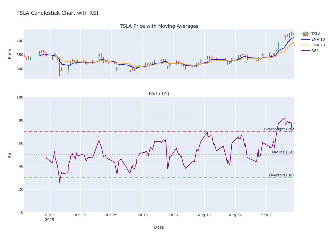
We have calculated and plotted EMAs and RSI..Now, let’s generate signals
Before I do this, allow me to share what the rules are.
We only take a trade when BOTH indicators agree on the same direction. Think of it as getting confirmation from two different sources before making a decision.
Bullish (BUY) Signal Rules:
- Moving Average Condition: The fast EMA (10) must cross ABOVE the slow EMA (20)
- RSI Condition: RSI must be above 50 AND rising (or crossing above 50 around the same time)
- Both must happen: We need BOTH conditions within a few candles of each other
Why this works: The EMA crossover tells us the trend might be turning bullish, while RSI above 50 and rising confirms that momentum is actually building upward.
Bearish (SELL) Signal Rules:
- Moving Average Condition: The fast EMA (10) must cross BELOW the slow EMA (20)
- RSI Condition: RSI must be below 50 AND falling (or crossing below 50 around the same time)
- Both must happen: Again, we need BOTH conditions to align
Why this works: The EMA crossover suggests a bearish trend change, while RSI below 50 and falling confirms downward momentum is actually taking hold.
def calculate_signals(df):
    """Calculate buy/sell signals based on RSI + EMA strategy"""
    df['Signal'] = 0
    df['Signal_Type'] = ''

    # Calculate EMA crossovers
    df['EMA_Cross'] = 0
    df['EMA_Cross'] = (df['EMA_10'] > df['EMA_20']).astype(int) * 2 - 1  # 1 for bullish, -1 for bearish
    df['EMA_Cross_Signal'] = df['EMA_Cross'].diff()

    for i in range(1, len(df)):
        # Bullish signal: EMA10 crosses above EMA20 AND RSI confirms
        if (df['EMA_Cross_Signal'].iloc[i] == 2 and  # EMA bullish cross
            df['RSI'].iloc[i] > 50 and  # RSI above midline
            df['RSI'].iloc[i] > df['RSI'].iloc[i-1]):  # RSI rising

            df.loc[df.index[i], 'Signal'] = 1
            df.loc[df.index[i], 'Signal_Type'] = 'BUY'

        # Bearish signal: EMA10 crosses below EMA20 AND RSI confirms
        elif (df['EMA_Cross_Signal'].iloc[i] == -2 and  # EMA bearish cross
              df['RSI'].iloc[i] < 50 and  # RSI below midline
              df['RSI'].iloc[i] < df['RSI'].iloc[i-1]):  # RSI falling

            df.loc[df.index[i], 'Signal'] = -1
            df.loc[df.index[i], 'Signal_Type'] = 'SELL'

    return df

def visualize_with_signals(df, title="TSLA Strategy with Buy/Sell Signals"):
    """Enhanced visualization with buy/sell signals"""
    fig = make_subplots(
        rows=2, cols=1,
        shared_xaxes=True,
        vertical_spacing=0.1,
        subplot_titles=('TSLA Price with Signals', 'RSI (14)'),
        row_width=[0.7, 0.3]
    )

    # Add candlestick chart
    fig.add_trace(go.Candlestick(
        x=df.index,
        open=df['Open'],
        high=df['High'],
        low=df['Low'],
        close=df['Close'],
        name='TSLA'
    ), row=1, col=1)

    # Add EMAs
    fig.add_trace(go.Scatter(
        x=df.index, y=df['EMA_10'],
        mode='lines', name='EMA 10',
        line=dict(color='blue', width=2)
    ), row=1, col=1)

    fig.add_trace(go.Scatter(
        x=df.index, y=df['EMA_20'],
        mode='lines', name='EMA 20',
        line=dict(color='orange', width=2)
    ), row=1, col=1)

    # Add buy signals
    buy_signals = df[df['Signal'] == 1]
    if not buy_signals.empty:
        fig.add_trace(go.Scatter(
            x=buy_signals.index,
            y=buy_signals['Close'],
            mode='markers',
            marker=dict(symbol='triangle-up', size=15, color='green'),
            name='BUY Signal'
        ), row=1, col=1)

    # Add sell signals
    sell_signals = df[df['Signal'] == -1]
    if not sell_signals.empty:
        fig.add_trace(go.Scatter(
            x=sell_signals.index,
            y=sell_signals['Close'],
            mode='markers',
            marker=dict(symbol='triangle-down', size=15, color='red'),
            name='SELL Signal'
        ), row=1, col=1)

    # Add RSI
    fig.add_trace(go.Scatter(
        x=df.index, y=df['RSI'],
        mode='lines', name='RSI',
        line=dict(color='purple', width=2)
    ), row=2, col=1)

    # RSI reference lines
    fig.add_hline(y=70, line_dash="dash", line_color="red", row=2, col=1)
    fig.add_hline(y=30, line_dash="dash", line_color="green", row=2, col=1)
    fig.add_hline(y=50, line_dash="dot", line_color="gray", row=2, col=1)

    # Update layout
    fig.update_layout(
        title=title,
        xaxis_rangeslider_visible=False,
        height=800,
        showlegend=True
    )

    fig.update_yaxes(title_text="Price", row=1, col=1)
    fig.update_yaxes(title_text="RSI", range=[0, 100], row=2, col=1)
    fig.update_xaxes(title_text="Date", row=2, col=1)

    fig.show()
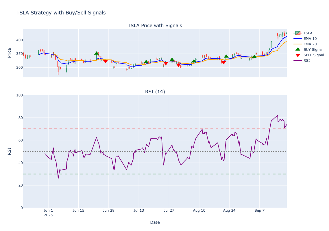
We have calcualte_signals to calculate signals 1 for Bullish and -1 for Bearish. When it is plotted, it looks like the below:
Conclusion
We’ve successfully built a multi-signal trading strategy that combines RSI and Moving Average crossovers for better signal quality. By requiring confirmation from both indicators, we filter out many false signals that would occur when using either indicator alone. This systematic approach provides a solid foundation for identifying higher-probability trading setups across different timeframes and assets. Like always, the code is available on GitHub
Looking to create something similar or even more exciting? Schedule a meeting or email me at kadnan @ gmail.com.
Love What You’re Learning Here?
If my posts have sparked ideas or saved you time, consider supporting my journey of learning and sharing. Even a small contribution helps me keep this blog alive and thriving.